How to work in the statistics program. Free programs for statistical data analysis
Overview of statistical programs
At the stage of planning an experiment, the functions from the Sampling menu will be useful for the researcher, allowing you to determine the required number of groups for some of the most common research tasks. Among the functions implemented in MedCalc, special mention should be made of the ability to carry out basic types of statistical analysis, without having sample values, i.e. based on average values, scatter indicators, etc. This can be useful when studying literature data, since complete information the primary results of the experiment are not reported in publications. For example, to compare sample means using the Student's test, it is enough to know the arithmetic means themselves, the standard deviation and the sizes of both samples. This data should be entered in the window called Tests > Comparison of >
Title: Review statistical programs
Detailed description:
The productivity of the work performed is closely related to the tools used. So, according to legend, Archimedes said that he could turn the Earth over if he received the necessary fulcrum and leverage. But the great philosopher did not have the necessary tools, and our planet is still flying in its orbit. A similar situation arises in the field of statistical analysis of research results. It is quite possible to carry out statistical data processing with only a pencil and paper, but it is much faster and more efficient to do this with the help of special tools, namely statistical software. Strictly speaking, software packages used for statistical analysis should be classified as math programs Therefore, in this article the terms “mathematical” and “statistical” will be used interchangeably.
As a rule, young scientists take their first steps in statistics using spreadsheet processors, with the vast majority using MS Excel. Second most popular table processor for today - Calc from office suite OpenOffice.org. Unfortunately, some researchers perceive these programs as the most convenient and suitable tool for analysis. However, they are mistaken. The use of such software is permissible in cases where it is necessary to perform simple operations such as sorting data, calculating descriptive statistics, constructing certain types of graphs, and also simply to save the primary data of your experiment and keep a laboratory journal. In other words, full statistical processing of research results in Excel is impossible. This is an office application, not a scientific one.
All scientific mathematical applications can be divided into two large groups: programs with graphical interface and without it. You should not think that the graphical interface somehow characterizes the quality software product. These properties are in no way dependent on each other. However, such a division has a huge practical significance. The fact is that not everyone can comfortably work on the command line. Today, many computer users do not even think about abandoning the “cliquedromes” on which an impressive part of the modern IT industry rests. However, it is still more convenient to perform mathematical calculations by typing commands from the keyboard rather than clicking on numerous buttons on the screen. Therefore, in serious applications there is a mode command line with built-in programming language and graphical interface.
First, let's get acquainted with the statistical computing environment and the programming language R. Its origins lie in the S programming language, with which they have a lot in common. The standard package of R does not include a graphical interface, which is familiar to many users. As a result, a number of researchers have the erroneous opinion that this tool Allows you to perform numerical calculations only, but does not have graphing capabilities. This is wrong. The R system has ample opportunities For statistical processing data, including for working with graphics, and the window interface can be set as additional application. But it should be borne in mind that graphic user interfaces for R are noticeably inferior to those in other statistical packages.
You can install the R environment on a computer running Windows control, MacOS or Linux. When starting the R system, an inexperienced user will have the question: “Where should I enter data?” Due to the lack of a built-in table editor, the analyzed information is either entered directly into the command line as an argument to the corresponding functions, or loaded from external files. The first option is convenient when working with single values, and the second - in cases where it is necessary to work with tables. The tables themselves can be created in any spreadsheet processor, and the files can be saved in *.csv format, which is easily loaded into R.
Having loaded the information into variables, you can begin to process it using huge amount functions implemented in R. But it should be remembered that all intermediate data when working with this language is stored not in temporary files, but directly in RAM. This feature must be kept in mind when processing very large volumes Information: R will use a significant portion of the computer's RAM.
The syntax of the language is quite simple and easy to learn. To date, more than a hundred books have been written on various areas of using the R statistical computing environment, but all of them are based on English. Unfortunately, there is still very little information in Russian and it is presented only in the form of scattered articles on some issues of use of this language programming. It is the lack of information that is holding back the spread of a high-quality software package in our country (despite the fact that it is free).
The R's reliability comes from its origins. Language was created as free implementation Very powerful language programming S, the history of which dates back to 1976, when the first working version. Today the S language is the basis S-PLUS applications, developed by TIBCO Software Inc., and, unlike R, is commercial product. S-PLUS has a nice graphical interface, in which data can be entered by loading from an external file, database, or by copying a table from text file, or a table processor. S-PLUS, like R, can run on different operating systems and can be used to perform numerical and graphic methods analysis.
Another popular one statistical application is a SAS system that originated in the 1960s at the University of North Carolina as an application for analyzing agricultural research results. Today, the system continues to be developed by the SAS Institute, which has already released the ninth version of this program. The scope of application of SAS is very diverse scientific research, business analyst, etc.
The system consists of modules, each of which performs a specific range of tasks. The BASE and STAT modules are most often used in statistical processing. The SAS system implements its own programming language, which in its syntax is closer to BASIC and is not similar to R or S. The system allows you to load data from external files or enter them directly into the terminal window. Working with SAS, you can carry out statistical processing of data of different levels of complexity, in accordance with the assigned tasks. Interaction with the program is possible both in console mode and through a graphical interface, which is graphical shell for simplified input of SAS programming language commands.
Programs that primarily use the command line interface also include Stata, developed by the American corporation StataCorp. The application can run on operating systems Windows family, on MasOS and Linux. Data entry here is possible either by loading from external files or using the built-in table editor, which is quite simple, but allows you to perform all the necessary manipulations with tables. The principles of working with the Stata application are no different from those when using the programs described above. Those users who find terminal mode inconvenient can use the program menu to automatically generate built-in programming language commands.
All described statistical packages can be used for any type of statistical analysis. Thus, the functionality of the R language can be changed by adding libraries of functions that are strictly oriented certain type tasks. In addition, anyone who has enough knowledge and experience with this language can create native functions and libraries that correspond to the specifics of a particular user’s work.
But in addition to “general profile” statistical software, there are programs aimed at scientists working in the field of biomedical research. Thus, the MedCalc program, developed since 1993 by the Belgian company MedCalc Software, is positioned as a full-fledged statistical application created in accordance with the needs of biomedical researchers. The developers focus the attention of researchers on the ease of use of MedCalc for analyzing ROC curves.
The program is convenient in that it does not offer redundant functionality, which often confuses an unprepared person starting to work with universal applications. In addition to this, the ability to work only in a graphical interface without using the command line makes the program less flexible, but more attractive for use in this field of science, since specialists with medical education very rarely can boast of extensive experience working with mathematical programs.
To date, the twelfth version of the program has been created. Unfortunately, only Windows users, but this disadvantage is compensated by relatively small system requirements and the ability to run the application in both Windows 2000 and Windows 7. For those who have never used the program, it is possible to download a fully functional demo version of the product from the medcalc.org website, which will work without restrictions for fifteen days. In addition, the package includes demo files containing data sets and examples of their analysis.
Data entry into MedCalc is carried out in an integrated spreadsheet editor or by importing files various formats, such as *.csv, excel, etc. To call the built-in editor, just select the Spreadsheet command in the menu, after which you can start generating a table. In statistical programs, the columns of tables are called “variables” and the rows “cases.” When creating a table, it will be useful to follow several rules:
. The first variable must contain the serial numbers of the cases. This is necessary in order to be able to restore their previous order after re-sorting the values.
. Numerical values should be entered without rounding to avoid losing information.
. If some values are missing, you can skip them, leaving empty cells in the table.
. Each variable must have only one value for each case.
After saving the table or loading a file with data, the information processing stage begins. To perform statistical analysis, select the appropriate item in the Statistics menu. Each type of analysis has its own set of settings, for which you can get help by clicking the Help button.
At the stage of planning an experiment, the functions from the Sampling menu will be useful for the researcher, allowing you to determine the required number of groups for some of the most common research tasks. Among the functions implemented in MedCalc, special mention should be made of the ability to conduct basic types of statistical analysis without having sample values, i.e. based on average values, scatter indicators, etc. This can be useful when studying literature data, since complete information about the primary results of the experiment is not provided in publications. For example, to compare sample means using the Student's test, it is enough to know the arithmetic means themselves, the standard deviation and the sizes of both samples. This data should be entered in the window called Tests > Comparison of > means (t-test), and the comparison result will be displayed in the same window. The rest of the functions in the Tests menu are used in the same way.
Thus, the MedCalc program provides the user with user-friendly interface without excessive “functionality”, equipped with good spreadsheet editor. All calculations and diagrams are saved in one file and are easily sorted into special list on the left side of the main program window. Statistical analysis is performed using conveniently organized menus, equipped with concise and understandable reference material. In this regard, the program will be very useful for scientists performing biomedical research and inexperienced in mathematical applications.
MedCalcl is a simple and easy-to-use program, but not every user can get everything he needs to do his job from it. Among those who place very high demands on statistical software and are willing to shell out several thousand dollars for it, applications such as Statistica or SPSS Statistics are popular. Both programs are real “monsters” in comparison with MedCalc - both in cost and in their computing capabilities. It is impossible to talk about them in detail within the framework of an article; for this you would have to write a book of several hundred pages, so we will limit ourselves to a brief introduction.
Statistica is developed by StatSoft. To date, the latest version is Statistica 9. The SPSS program, whose name is an abbreviation for Statistical Package for the Social Sciences, relatively recently became owned by IBM and changed its name to PASW (Predictive Analytics SoftWare) Statistics. Both programs have an excellent graphical interface, a built-in programming language and the ability to integrate with the statistical computing language R.
It should be noted that almost limitless possibilities in statistical processing, provided by these tools, require large computer resources. Thus, SPSS requires at least 1 GB of RAM to run. Operating systems, in which you can run SPSS: Windows, MacOS and Linux. Statistica is developed only for Windows, which somewhat reduces the number of its users.
As always, work in programs begins with data entry. The integrated table processor allows you to design tables using familiar formats for each user. office applications ways. Saved tables, as well as calculation results, graphs and reports in Statistica can be conveniently located in one file called “ Workbook”, while the workspace organization in SPSS is less convenient, but still quite acceptable for use after a short adaptation period.
The programs contain all the most popular statistical methods: frequency analysis, calculation statistical characteristics, contingency tables, correlations, plotting, t-tests and large number nonparametric tests, multivariate linear regression analysis, discriminant analysis, factor analysis, cluster analysis, variance analysis, reliability analysis, multidimensional scaling and a number of others. Calling these statistical procedures is done by selecting the corresponding windows from the menu and entering into them necessary settings. All types of analysis are divided into groups, which helps you quickly navigate the application interface.
The STATISTICA and SPSS systems have extensive graphic capabilities. They include a wide variety of categories and types of charts, including scientific, business, 3D and 2D charts in various systems coordinates, specialized statistical graphs— histograms, matrix, categorized graphs, etc.
The statistical functions available in both applications are striking in their variety. It seems that these statistical analysis tools allow you to do anything, provided that the user has thoroughly studied how they work. The main obstacle to mastering these programs is the time that needs to be spent on training. It is precisely because of the user’s lack of knowledge that, in most cases, the power of statistical packages of this level is not even half used.
As you can see, there are many applications for statistical analysis in the world. Only a small part of them was briefly described in this article. Outside of it there were such programs as Minitab, MatLab, Octave, GenStat, JMP, Analyse-it, domestic development STADIA and many other, large and small, expensive and free programs. However, such an abundance of software should not frighten the researcher; it will be enough to once make a thoughtful choice in favor of one or two programs, carefully study the intricacies of their use, and they will serve for many years faithful assistants in statistical analysis of experimental results.
STATISTICA is a system for statistical data analysis, including a wide range of analytical procedures and methods:
more than 100 various types graphs, descriptive and within-group statistics, exploratory data analysis, correlations, quick basic and block statistics, interactive probability calculator, T-tests (and other group difference tests), frequency, contingency, flag and header tables, multivariate response analysis, multiple regression, nonparametric statistics, general model analysis of variance and covariance, distribution fitting, data mining, neural networks and much more. STATISTICA series products are based on the most modern technologies, fully comply with the latest achievements in the field of IT, allow you to solve any problems in the field of data analysis and processing, ideal for solving practical problems in marketing, finance, insurance, economics, business, industry, medicine, etc.
Comsol Multiphysics 4.3
A program for finite element calculations of complex scientific and technical problems. COMSOL Multiphysics allows you to simulate almost anything physical processes, which are described by partial differential equations. The program contains various solvers that will help you quickly deal with even the most complex tasks, A simple structure The application provides ease and flexibility of use. The solution to any problem is based on the numerical solution of partial differential equations using the finite element method. The range of tasks that can be modeled in the program is extremely wide.
The set of special modules in the program covers almost all areas of application of partial differential equations.
COMSOL Multiphysics (Femlab) is a simulation package that solves systems of nonlinear differential equations partial derivatives using the finite element method in one, two and three dimensions. It allows you to solve problems in the field of electromagnetism, elasticity theory, dynamics of liquids and gases, and chemical gas dynamics. Femlab also makes it possible to solve the problem both in a mathematical formulation (in the form of a system of equations) and in a physical one (choice physical model, for example models of the diffusion process). Of course, in any case, a system of equations will be solved, and the difference lies only in the ability to use physical systems units and physical terminology. In the so-called physical mode of operation, it is also possible to use predefined equations for most phenomena found in science and technology, such as heat and electricity transfer, elasticity theory, diffusion, wave propagation, and fluid flow.
STATISTICA
Year/Date of Issue: 2011
Version: 10.0.1011
Bit capacity: 32bit
Vista Compatibility: full
Windows 7 compatibility: full
Interface language: English
Tablet: Present
Comsol Multiphysics 4.3
Year/Date of Issue: 2012
Version: 4.3 build 151 (build 184 if you install Update1)
Bit depth: 32bit and 64bit
Compatible with Vista and Windows 7: full
Interface language: English
Tablet: Present
Build Size: 5.18 GB
How to fix problems:
1. If there is a problem with the license (during installation or startup) and you are working via remote desktop ( remote desktop) then try using Radmin.
2. If nothing is displayed in the main window, try changing Options -> Preferences -> Graphics -> Rendering to something else (the default is OpenGL, i.e. usually you need to change to DirectX ... you can also to Software but it's slower).
Briefly about how to perform basic actions in the programStatistica 6.0
Preparing data for processing
All data must be presented in table form.
Each row of the table represents one study participant. That is, if a total of, for example, 42 people were examined (both experimental and control groups together), then the table contains 42 rows plus headings.
Each table column is a variable.
When preparing data variable We will consider any information about the study participant. For example, the first variable - the first column of the table - can become serial number or even some unique name test subject. The name itself is NOT required in the study. It can only be useful to accurately and accurately enter all the information about this particular person.
The next variable could be group type– experimental or control. You can call the variable “group”. This variable must be completed for all study participants. Please note: the SAME designation must be used for all participants in the SAME group. For example, exp.g.– for all participants in the experimental group, counter.g.– for all participants in the control group. Next, you can specify the gender of the study participants.
In the example data file, the first variable is Pol. The next variable is age. Here the age is simply indicated in years. Next comes the variable Edu – level of education. This variable can take only 3 values - “secondary-specialized,” “higher,” “incomplete higher.” The following is the length of service in years. The next variable, marital status, can also take on several values. In this example, the first six variables contain general sociodemographic information; These are not techniques yet.
The next three variables - No. 9, 10, 11 - correspond to three scales of the Maslach methodology (the names of the scales are not important to us now). Each of them can take values from 0 to a certain level, now this is not important.
Variables 12, 13 and 14 – assessments of the components of the socio-psychological climate: emotional, cognitive and behavioral components. Calculated according to the method. Can only take three values -1, 0, 1.
In total, in our example we get 14 variables.
I draw your attention to the fact that the variables are different. We will be primarily interested in dividing the variables into metric And nominative. Metric variables - for example, age, intelligence scores, etc. - can take on different values within a certain range, with a higher or lower value corresponding to a higher or lower value. to a lower level measured characteristic.
Nominative variables can take a fixed number of values. For example, the variable “gender”. It can take two values – M or F. The variable “level of education”: can take three values – secondary vocational, higher, incomplete higher. The “group type” variable is also nominative; it specifies whether the participant belongs to the experimental or control group.
Question: determine which variables from your research are metric and which are nominative. This is extremely important for the choice of research methods.
The result this stage work is a table with data (compiled on paper or - better - in Excel), plus an understanding of which variables are metric and which are nominative.
Creating a new file in the programStatistica 6.0
Open the program and select File–New from the top menu. (I recommend using the English version of the program)
A window will appear in which you can select the required number of variables (NumberofVariables) and the number of observations (NumberofCases). In our example there will be 14 variables and 78 observations. Click OK.


We get clean file, into which you can enter research results. This sheet may not be completely visible, so there are scroll bars at the bottom and right.
The result of this stage is a blank sheet on which the research results can be entered.
An example of such a sheet is below.

Data entry
If you created a data table in Excel, you can copy the data from there into statistics.
(Generally speaking, the Statistica program supports importing data from Excel, but for this you need to organize the data very correctly and perform the import itself very correctly. You can make mistakes. Therefore, I suggest transferring the data “manually.”)
How to create variable names
When creating a new file, all the variables in it are already signed and are called Var1, Var2, Var3, etc. To make it more convenient to work, you need to rename them. To do this, double-click on the variable headers l eva To foot m yushki (designation – 2LKM). A window will open. In it, click on the “AllSpecs...” button, as shown in the figure.

A window will open in which you can label all variables.

After that, click OK. The names of the variables that you write will appear instead of Var1, etc. The numbering of variables will remain, and this is normal.
Next, you need to fill out the entire table with data. If you have already entered data into the Excel program, then you can select a range with data there (without any numbering and without variable names), copy it, and paste it into the Statistica program.
After this, it is advisable to save the data file: menu File–SaveAs..., then specify where to place this file and what to call it. The program writes the file type automatically. To save, click the “Save” button. After saving the file, its name appears on the screen, on blue background in the title line. It looks something like this:

The result of this stage is a completed and saved file with the research results.
Calculations in the program
From now on, the most useful item in the top menu is Statistics.
Comparison of means in two groups - Student's T-test
This criterion can be used to compare the average values of ONLY metric variables and ONLY in TWO groups (not three, four, ...)
In our example, the variables are metric:
No. 3 – Age – age
No. 5 – Stajj – work experience
No. 7 – ProfStress – an indicator of professional stress
No. 9 – Maslach_1 – the first indicator of the Maslach method
No. 10 – Maslach_2 – the second indicator of the Maslach method
No. 11 – Maslach_3 – the third indicator of the Maslach method
The “Gender” variable divides all participants into two groups – men and women.
The “Group” variable divides all participants into two groups – the experimental group and the control group.
Accordingly, in our example, using the Student's T-test, we can check whether 1) the average values of the variables listed above differ between men and women; 2) whether the mean values of the above variables differ between participants in the experimental and control groups.
IN top menu select Statistics – in it Basic Statistics/Tables.

 select, click OK.
A window with settings appears. First of all, we need to select the variables for which we want to carry out the calculation. To do this, click the Variables button as shown in the figure:

The variable selection window appears.

Here on the left side – Dependentvariables – you need to indicate those metric variables whose average values we want to compare. For example, these are variables 3, 5, 7, 9-11 (age, experience, stress, etc.). You can select variables from the list or type numbers in an empty window.
On the right side – Groupingvariable – we indicate ONE variable that divides our sample into two groups. For example, you can select the 1-Pol variable, then we will compare the indicators of men and women. Or you can select the 2-Group variable here, then we will compare the experimental and control groups. If we are interested in both options, we will have to apply the T-test twice. But only one variable is selected at a time on the right side of the window.
Now let's look at an example with the 1-Pol variable. It will look like this:
 Now OK.
The program returns us to the previous window. To perform calculations, you need to click the Summary button, one of the two, they are shown in the picture.

Another window will appear on the screen – Workbook1. The program will write all calculation results to this file.

Let us consider the results obtained in detail.

In the table on the left at gray background The variables whose mean values we compared are listed. The columns “Meanж” and “Meanм” contain the average values of the variables for women and men, respectively. That is, the average age of women is 40.68, the average age of men is 39.15 years. The average length of service for women is 17.44 years, for men – 16.87 years. Next, the t-value column contains the value of the t-criterion; we don’t need it. The df column denotes the number of degrees of freedom; we don’t need that either. (That is, when presenting the results of statistical data processing in work, it would be nice to indicate these numbers, but there is no need to decipher them). The next column –p– is required. This is the same level of reliability of differences in average values. Probably the most important column from this table.
Theoretical digression. To test whether the means of the two groups are different, we first calculate these values. And almost always the average values in the two groups will be at least somewhat different. That is, we almost always get DIFFERENT average values. In our example it’s the same – the average values for women and men for all variables are different. But in some places they differ more, in others less. And “by eye” we cannot determine whether the average values differ “a little” or “a lot.” This can only be determined using statistical tests, for example, Student's t-test.
Without going into details of the calculations, I suggest you remember:
Average values in two groups for any variable significantly different,If indicator p<0,05 (in the program these variables are highlighted in red)
In this case, they also say that the differences in mean values are reliable (or statistically significant) at the 5% level.
Sometimes, if p is greater than 0.05 but less than 0.1, then the differences are said to be at the level of a statistical trend. That is, these are less pronounced differences.
But usually if p>0.05, then they say that no significant differences have been identified/not established/not found. But EVEN IF p>0.1, YOU CANNOT SAY THAT THE AVERAGE VALUES ARE THE SAME.
Thus, in in this case for men and women, only indicators of professional stress differ significantly (p value = 0.029, this is less than 0.05). At the trend level, there are differences in the Maslach_2 indicator (here p = 0.051, this is more than 0.05, but less than 0.1). No significant differences were found for other variables.
Now let's look at a comparison of the average values in the experimental and control groups.
Again in the top menu, select Statistics – in it BasicStatistics/Tables. Since we have already launched this program module, a window will appear on the screen

You can select "Continuecurrent" to continue the calculation.
To jump to a comparison between the experimental and control groups, click the Variable button. In the right part of the window –Groupingvariable– select variable number 2. Click OK. ClickSummary as in the pictures above.
We get the following result.

Please note that for the participants in the experimental and control groups the average age, average length of service and average values for the Maslach_2 indicator are significantly different. No significant differences were found for other variables.
How to close the program.

First you need to close all calculations. To do this, click on the rectangle in the lower left corner, a calculation window will open, close it with a cross or the Cancel button.
The second step is to close the Workbook1 window – also with a cross. You can save this file, but it is not necessary.
The third step is to close the data file.
Fourth, close the program.
I'll add later:
Comparison of means in two groups is a non-parametric method.
Comparison of means in three or more groups - analysis of variance
Analysis of contingency tables - Chi-square.
Using the Chi-square criterion, we find that the distribution according to the attribute “like/dislike ice cream” among boys and girls is significantly different. That is, they have “different” attitudes towards ice cream.
Here, using Chi-square, we find that no significant differences were found. That is, boys and girls “do not differ” in their love/dislike for computer games.
We check whether the educational level of participants in the experimental and control groups differs.


Correlation coefficients.
Transferring results to Excel
Along with commercial statistical packages, there are quite a few large number completely free statistical programs and applications. At the same time, a number of free programs are not only not inferior, but even superior in functionality to commercial applications. I will give a list of the main free programs for statistical data processing.
ξ EpiInfo - free statistical package, the development of which is supported by the US Centers for Disease Control. The main feature is the ability not only to conduct statistical analysis, but also to create questionnaires and forms for data entry (including the creation of forms for collecting information on the Internet). Latest version also supports integration with Google Maps and visualization of cartographic information. A rather significant limitation for large data sets can be the use as a database Microsoft format Access.
ξ OpenEpi- kit statistical functions, allowing you to quickly apply relatively simple and commonly used statistical tests. OpenEpi can be used online on the developer’s website, or installed on your computer. The advantage of the package is a set of functions for calculating statistical power, number of groups, generation random numbers, as well as the ability to calculate statistical significance based on group statistics, which can be useful when evaluating articles.
ξ PSPP- By appearance and functionality is very reminiscent of SPSS (in fact, the name of the package is mirror image), and is completely free.
ξ SOFA — Allows you to perform basic statistical tests, but does not allow you to perform regression analysis. One of distinctive features package is quick creation various standard graphs and summarizing tables that do not require formatting, as well as the ability to execute custom scripts in Python.
ξSEER-Stat is a free statistical package aimed at application in oncology, the development of which is supported by the US Cancer Institute. IN software package many functions for calculating morbidity, survival and mortality (including age-standardized indicators).
ξWINPEPI— a program for analyzing epidemiological data. Detailed description functionality is located . The same author created a number of other programs for use in epidemiology.
ξ Statistical Analysis for Genetic Epidemiology is a statistical analysis program for geneticists and epidemiologists, which contains many functions for obtaining descriptive statistics, data verification, quantification heredity of a trait or disease, assessment of the most likely age of onset of the disease, identification of patterns of occurrence of individual alleles or single-nucleotide changes, and other possibilities.