Programs for automatically filling out forms. Autofill cells and copy formulas in Excel

Autofill in Excel is a very convenient function that makes it much easier to both fill tables with data and work with calculations and formulas.

Autocomplete is used in the following situations:

• Copying data to adjacent cells (for example, when filling a table, all cells in a column have the same value)
• Filling a column or row with data that changes at a certain interval (for example, row numbering)
• Copying formulas (for example, the price and quantity of an item are indicated in two columns; to calculate the order amount for each item, just count it in one cell and copy the formula for the entire column)

How to autocomplete in Excel?

Copying data in adjacent cells

To fill adjacent cells with the same data, do the following:

• Hover your mouse over the lower right corner of the cell until the “ + »
• Hold the left mouse button and drag in the desired direction to fill the cells with data

The second way to autocomplete in Excel:

• Enter the required data in the first cell
• Select a cell to the right, left, bottom, or top of the data cell
• Click the Fill button on the toolbar (Home Tab)
• Select direction (up, down, left or right)

Filling adjacent cells with a sequence of data (numbers, text, inline lists)

In order to automate data entry into cells, you can use built-in lists, as well as autocomplete sequences. For example:

How to autofill such data in an Excel table?

• Enter the required data in the first two cells
• Select two cells with data, move the mouse cursor to the lower right corner so that the “+” sign appears
• Hold down the left mouse button and drag in the desired direction

For the convenience of working with tables, you can create such a list yourself. For example, with the names of employees. In order to then enter them into the column, one surname (which is first in the list) will be enough.

To create a list like this:

The list will be saved in Excel settings

Copying formulas in Excel

In order to copy the formula, you must do the following:

• Enter the formula in the first cell
• Select cell with formula
• Hover the mouse cursor over the lower right corner of the cell so that the “+” sign appears
• Hold down the left mouse button and drag in the desired direction

Excel is one of the best editors for working with tables today. This program has all the necessary functions to work with any amount of data. In addition, you will be able to automate almost every action and work much faster. In this article we will look at in what cases and how exactly you can use cell autofill in Microsoft Office Excel.

It is worth noting that such tools are not available in Microsoft Word. Some people resort to trickery. Fill the table with the required values ​​in Excel, and then transfer them to Word. You can do the same.

Setting up automatic numbering is very easy. To do this, just take a few very simple steps.

1. Dial some numbers. Moreover, they must be in the same column or one line. In addition, it is desirable that they go in ascending order (order plays an important role).

1. Highlight these numbers.
2. Hover over the bottom right corner of the last element and drag down.

1. The further you pull, the more new numbers you will see.

The same principle works with other values. For example, you can write several days of the week. You can use both abbreviated and full names.

1. Let's highlight our list.
2. Move the cursor until its marker changes.
3. Then pull down.

1. As a result, you will see the following.

This feature can also be used for static text. It works exactly the same.

1. Write a word on your sheet of paper.
2. Pull the lower right corner down a few lines.

1. You'll end up seeing a whole column of the same content.

In this way, you can make it easier to fill out various reports and forms (advance, KUDiR, PKO, TTN, and so on).

Ready-made lists in Excel

As you can see, you are not asked to download any free add-ons. All this works immediately after installing Microsoft Excel.

Creating your own lists

The examples described above are standard. That is, these enumerations are set in Excel by default. But sometimes there are situations when you need to use your own templates. It's very easy to create them. To set up, you need to perform a few very simple manipulations.

1. Go to the "File" menu.

1. Open the Settings section.

1. Click on the “Advanced” category. Click on the "Edit Lists" button.

1. After this, the “Lists” window will open. Here you can add or remove unnecessary items.

1. Add some items to the new list. You can write whatever you want - it's your choice. As an example, we will write a list of numbers in text form. To enter a new template, click on the “Add” button. After this, click on “OK”.

1. To save the changes, click “OK” again.

1. Let's write the first word from our list. You don't have to start from the first element - autocomplete works from any position.

1. Then we will duplicate this content several lines below (how to do this was written above).

1. As a result, we will see the following result.

Thanks to the capabilities of this tool, you can include anything in the list (both words and numbers).

Using progression

If you are too lazy to manually drag the contents of the cells, then it is best to use the automatic method. There is a special tool for this. It works as follows.

1. Select any cell with any value. We will use the cell with the number “9” as an example.
2. Go to the Home tab.
3. Select "Progression".

1. After this you can configure:
   • filling location (by rows or columns);
   • progression type (in this case, choose arithmetic);
   • step of increment of new numbers (you can enable or disable automatic step detection);
   • maximum value.

1. As an example, in the “Limit value” column we indicate the number “15”.
2. To continue, click on the “OK” button.

1. The result will be as follows.

As you can see, if we had specified a limit greater than "15", then we would have overwritten the contents of the cell with the word "Nine". The only disadvantage of this method is that the values ​​may fall outside the boundaries of your table.

Specifying the Paste Range

If your progression went beyond the permissible values ​​and at the same time overwrote other data, then you will have to cancel the insertion result. And repeat the procedure until you find the final progression number.

But there is another way. It works as follows.

1. Select the required range of cells. In this case, the first cell should contain the initial value for autofill.
2. Open the Home tab.
3. Click on the "Fill" icon.
4. Select "Progression".

1. Please note that the “Layout” setting is automatically set to “By Columns” because we selected the cells that way.
2. Click on the "OK" button.

1. As a result, you will see the following result. The progression is filled to the very end without leaving anything out of bounds.

Autocomplete date

You can work with date or time in a similar way. Let's follow a few simple steps.

1. Let's enter any date in some cell.
2. Select any arbitrary range of cells.
3. Let's open the "Home" tab.
4. Click on the “Fill” tool.
5. Select the “Progression” item.

1. In the window that appears, you will see that the “Date” type has been activated automatically. If this does not happen, then you entered the number in the wrong format.

1. To insert, click on “OK”.

1. The result will be as follows.

Autocomplete formulas

In addition, you can copy formulas in Excel. The operating principle is as follows.

1. Click on any empty cell.
2. Enter the following formula (you will need to adjust the address to the cell with the original value).

1. Press the Enter key.

1. Then you will need to copy this expression to all other cells (how to do this was described a little higher).

1. The result will be as follows.

Differences between Excel versions

All the methods described above are used in modern versions of Excel (2007, 2010, 2013 and 2016). In Excel 2003, the Progression tool is located in a different section of the menu. In all other respects, the operating principle is exactly the same.

In order to set up cell autofill using progression, you need to perform the following very simple operations.

1. Go to any cell with any numerical value.
2. Click on the "Edit" menu.
3. Select "Fill".
4. Then – “Progression”.

1. After this, you will see exactly the same window as in modern versions.

Conclusion

In this article, we looked at various methods for autofilling data in the Excel editor. You can use any option convenient for you. If suddenly something doesn’t work out for you, perhaps you are using the wrong data format.

Note that the values ​​in the cells do not need to increase continuously. You can use any progressions. For example, 1,5,9,13,17 and so on.

Video instructions

If you have any difficulties using this tool, you can also watch a video with detailed comments on the methods described above to help.

Autocomplete you can use it where you need to enter serial data. Let's say you need to fill a row or column with numbers, each of which is greater (or less) than the previous one by a certain amount. To avoid doing this manually, you need to do the following.

The formal algorithm looks like this.

1. Type the first two numbers in two adjacent cells so Excel can tell the difference between them.
2. Select both cells. To do this, click on one of them and, while holding down the mouse button, drag the selection frame onto the adjacent cell so that it captures it.
3. Hover your mouse over the marker located in the lower right corner of the selection frame (Fig. 2.26, a). At the same time, it will take the form of a black plus sign.
4. Click and hold down the mouse button and drag the frame until the last number to be inserted in the last cell appears in the tooltip near the mouse pointer. You can drag the frame in any direction (up-down, left-right) (Fig. 2.26, b).
5. Release the mouse button so that the range of covered cells is filled (Fig. 2.26, c).

The cells that I selected were filled according to the pattern. In the first column, 1 is added to the number in the previous line, in the second column - 2. Autofill can be used when entering time, dates, days of the week, months, as well as combinations of text and number. Look at fig. 2.27.

In this table, I just had to enter the first row, then select it and drag it down using the plus sign. Excel then increased each value by one. And if laboratory work did not take place every day, but every other day or every three days, then you would need to enter two lines for Excel to determine the difference between the values ​​​​in the cells. And then the program will fill in everything automatically, only it will increase the value in the cells not by one, but by the difference that you gave it (Fig. 2.28).

With AutoFill, you can copy the contents of a cell into a row or column. Take any cell, find the plus sign and drag it in any direction. In all cells to which you drag the selection, the first cell will be duplicated. Using the magic plus sign, you can copy not only the cell value, but also the cell data format.

For example, you entered time into a cell (that is, this cell is in the Time format) and you want the entire column to have exactly the same format. What to do? To do this, select the cell and drag the “plus” sign over the entire column. After you release the mouse button, the AutoFill Options button appears in the lower right corner of the row. By clicking on it, you will open a menu in which you can select the method of filling the cells (Fig. 2.29). Select Fill formats only. The entire column is now in Time format.

If you want to do the opposite, not save the format, but simply fill in the contents of the cells, select Fill in values ​​only. If you don't select anything, Excel will copy both the cell contents and format.

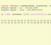
And I also want to draw your attention to the fact that Excel calculates decimal fractions to the 15th decimal place, but only two decimal places are displayed in the cells. The full number can be seen in the formula bar by selecting the cell (Fig. 2.30).

You can change the visible number of decimal places in the window shown in Fig. 2.25. Here you need to select number format options. By selecting any format from the list on the Number tab in the Format Cells window, you will read brief help about it and be able to change some settings.