How to set the cell size in Excel. Resize cells in Excel

Formatting and editing cells in Excel - handy tool for a clear presentation of information. Such possibilities of the program for work are invaluable.

There is no need to explain the importance of optimal data presentation to anyone. Let's see what can be done with cells in Microsoft Excel... From this lesson you will learn about the new possibilities for filling and formatting data in worksheets.

How to merge cells without losing Excel data?

Adjacent cells can be merged horizontally or vertically. The result is one cell that occupies a couple of columns or rows at once. The information appears in the center of the merged cell.

The order of combining cells in Excel:

The result will be:

If at least one cell in the selected range is still being edited, the button for merging may be unavailable. It is necessary to confirm the editing and press "Enter" to exit the mode.

How to split a cell into two in Excel?

Only a merged cell can be split into two cells. And an independent one, which has not been united, is impossible. BUT how to get a table like this:

Let's take a closer look at it in an Excel worksheet.

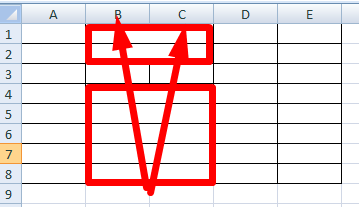
The line separates more than one cell, but shows the borders of two cells. Cells above "split" and below are concatenated by row. The first column, third and fourth in this table are made up of one column. The second column is of two.

Thus, in order to split the desired cell into two parts, it is necessary to merge adjacent cells. In our example, top and bottom. We do not merge the cell to be split.

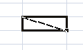
How to split a cell diagonally in Excel?

To solve this problem, you should perform the following procedure:

If you need to draw a diagonal in large cell, use the Insert tool.

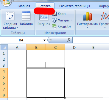
On the "Illustrations" tab, select "Shapes". Section "Lines".

We draw a diagonal in the desired direction.

How do I make the cells the same size?

You can convert cells to one size as follows:

You can change the width of cells throughout the sheet. To do this, you need to select the entire sheet. Left-click on the intersection of the row and column names (or the keyboard shortcut CTRL + A).

Move the cursor over the column names and make it look like a cross. Click on left button mouse and drag the border to set the column size. The cells in the entire sheet will become the same.

How do I split a cell into lines?

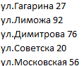
In Excel, you can make multiple rows from one cell. Streets are listed in one line.

We need to make several lines so that each street is written on one line.

Select the cell. On the "Alignment" tab, click the "Text Wrap" button.

The data in the cell is automatically spread across multiple rows.

Try it, experiment. Set the formats most convenient for your readers.

Most quick way to achieve that the contents of the cells are displayed in full - this is to use the mechanism of auto-fit the column width / row height according to the content.

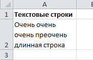
Let there be a table with cells filled with text values.

AutoFit Column Width

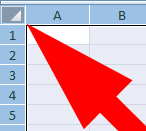
As you can see from the picture above, the text values ​​in the cells A2 and A3 are not displayed in full, because interferes with the text in the column B ... We need the content of all cells in the column A displayed in full. To do this, you need to make the column width A enough to display the longest text in the column. This is done very simply: move the mouse pointer to the column section A and B (on the gray header of the columns), the cursor will look like this:

We make a double click with the mouse and, Voila, the width of the column has become sufficient to display the values ​​in all cells of the column (taking into account the hidden rows).

If you need to align the width to the content of several columns at once, then we do the following:

• select the required columns (for their gray headings);
• move the cursor to any section of the selected columns and double-click.

Alternative option:

• Select the column or columns you want to resize;
• In the tab home in Group Cells select team Format;
• In Group Cell size select item AutoFit Column Width.

Auto-fit line height

If the cells contain values ​​with a very long line length (for example, if the length of a text line without hyphenation is comparable to the width of the visible part of the sheet), then the column width may become too large, and it will not be convenient to work with the data. In this case, you need to select the cells and enable the option Wrap by words across Cell format(or through the menu).

The column width remains the same, but the row height is automatically increased to fully display the cell value.

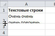
Sometimes, despite installed option Wrap by words, the line height is not enough to display text string completely (this could have happened if the line height was manually reduced). In this case, you need to do the same as we did in the case of selecting the row width - double-click on the section border, but now not columns, but rows:

Thereafter text value will be displayed in full in the cell:

Real example

Now we will apply the considered method in a real situation - we will edit the table created by copying data from MS ACCESS. We will copy through Clipboard some table from MS ACCESS to EXCEL sheet.

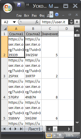
Note that the cells where we inserted the values ​​from Clipboard, option is enabled Wrap by words, although, by default, it is disabled (EXCEL itself enabled it on insertion). In addition, EXCEL did not change the default column widths, but only changed the row heights to fully display all values. Such table formatting does not always suit the user. Using the inserted table, we will solve 2 problems.

Task 1. Suppose we want all values ​​to be displayed in a table in one row.

For this:

• select the inserted values ​​(to do this, select any cell in the table and press CTRL + A(highlighted), if the table does not contain empty rows and columns, then all inserted values ​​will be highlighted);
• turn off the option Wrap by words(via the menu Home / Alignment / Text wrapping);
• the height of the cells will be reduced so that only one line is displayed, as a result, some of the values ​​will become invisible;

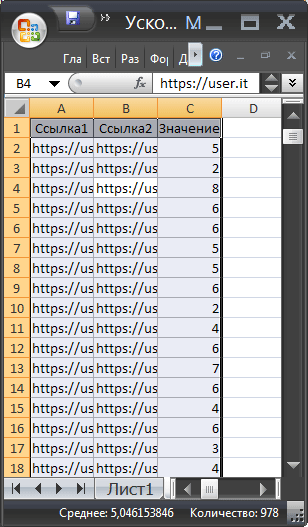
• highlight columns A , B and WITH for gray headings;
• hover over the column section A and B (on the gray header of the columns) and double-click.

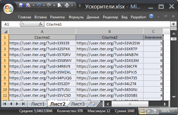
Task 2. Now, suppose we want all of the columns to have a specific user-defined width, and the values ​​are fully displayed in the cell. In this case, the line height should be minimal.

For this:

• set the columns width you want A , B and WITH ;
• option Wrap by words do not turn off (turn on);

• select all rows containing inserted values, or all sheet cells (all sheet cells can be selected by clicking the button Select all in the left upper corner sheet or double-clicking CTRL+ A);
• move the mouse pointer over any two filled-in rows section (on the gray column headings) and double-click.

Problem solved: the contents of all cells are fully displayed.

For any spreadsheet, not just a spreadsheet, cell height and width is one of the basic questions. What are, for example, various unified forms that are often implemented Excel tools... In this article, you will learn about how to size elements. spreadsheets(rows, columns, cells).

Let's consider several options:

• manual setting of borders;
• auto-fit depending on what is entered in the cell;
• precise dimensioning in selected units of measurement;
• using the clipboard;
• merging cells as a way to resize.

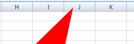
The first case is the most common. When you position the mouse cursor between the column names or row numbers, it changes shape to a double-headed arrow, the tips of which indicate in which directions the element can be resized.

The second option is best suited for a situation where you need to keep the row or column sizes as small as possible. Algorithm of user actions:

• select the element or several elements of the table for which the sizes are set;
• in the tab home expand the team's list Format and select the appropriate command auto-fit.

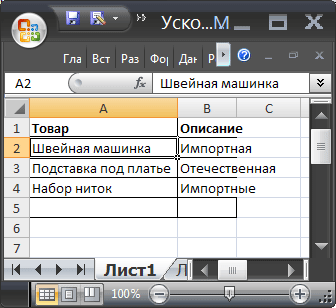
The result of auto-fitting the column widths can be seen in the figure.

For the various standardized tables, it is important to set the dimensions of the elements accurately. In this case, you first need to decide on the units of measurement. The default sizes are Excel sheets are given in inches. You can change these settings in the section Additionally commands Parameters in the tab File.

Changes are more clearly displayed in the mode Page layout(on the tab View find the appropriate command). The rulers become visible with markings in the selected units, for example, centimeters. Next, select the custom element (column or row) and set the size of the element (in the example, this is a column) using the corresponding command in the button menu Format.

If you need two elements of the same size, you can use Paste Special. To do this, you first need to copy the master element. Then select the element to which you want to apply formatting settings (including dimensions) and select Paste special in command options Insert, then in the dialog box - Column width.

The problem often arises to resize only one cell. This is possible in Word, but not possible in Excel, so you have to resort to a workaround, namely merging cells. This can be illustrated with the example of a uniform form. First, all columns are set to 1 mm wide, and then to the desired line a number of cells are selected and combined using the button Merge and center.

The combination of all resizing capabilities allows you to create the most complex tables, while retaining all the advantages of automating calculations in Excel.

Excel worksheet contains 1,048,576 rows and 16,384 columns. Filling in such a number of cells is very difficult and unnecessary. Often worksheets contain great amount information. To properly organize the structure of such data, it is important to be able to properly handle rows and columns - add, delete, hide, resize. Of course you can, but this is not always useful. This post is a must-read if you want to do some really serious tasks as you will be using row and column management a lot.

Insert new rows and columns

If the data on the worksheet is already organized, you may need to insert a blank row or column at a specific location.

To insert a line into a sheet, use one of two methods.

1. Select any cell in the row below the insertion point and run the command Home - Cells - Insert - Insert Rows to Sheet ... For example, if you need to insert a line between lines 3 and 4, place the cursor in any cell on line 4

1. Select the entire line before which you want to insert (to do this, click on the line number). Click right click mouse anywhere in the selected line and in the context menu select " Insert »

Both of these operations will lead to the emergence of a new empty line, the last line of the sheet will be deleted. If the last line (# 1 048 576) contains data, the program will not be able to insert new line and will give an error message. To fix this, delete or transfer information from the last line of the sheet.

Insert a new column in Excel is performed according to the same rules:

1. Place the cursor in any cell in the column to the right of the insertion point and execute: Home - Cells - Insert - Insert Columns to Sheet

1. Select the entire column in front of which you want to insert a new one, right-click anywhere in the selection, select the command “ Insert ».

When inserting a new column, the last one ("XFD") is deleted. If there is data in the last column, the insert will not be performed, the program will report an error.

Delete rows and columns in Excel

I always advise you to delete unnecessary information... If you have extra rows and columns on your sheet, you can delete them. I can offer 2 equivalent methods:

• Place the cursor in any cell of the row or column to delete and execute:
  • Home - Cells - Delete - Delete Rows from Sheet - to delete lines
  • Home - Cells - Delete - Delete Columns from Sheet - to remove columns

• Select the entire row or the entire column (by clicking on its number or name), right-click on the selected area and select "Delete" in the context menu

Deleting lines after context menu

When deleted, all subsequent rows are shifted up, and columns - to the left.

How to hide a row or column in Excel

If you want some rows and columns not to be visible on the screen, it is not necessary to delete them. They may contain important information, they can be referenced by formulas in other cells. It is better to hide such data from the eyes in order to simplify the structure of the sheet, leaving only the main thing. After hiding, all invisible values ​​are saved and participate in calculations.

I know 2 ways to hide:

• Place the cursor on any cell in the row or column to hide. On the ribbon, select:Home - Cells - Format - Hide or Show - Hide Rows(or Ctrl + 9), or Home - Cells - Format - Hide or Show - Hide Columns(or Ctrl + 0)

Hiding cells

• Select the entire row or column to hide, right-click on the selected area, select " Hide »

To display hidden cells again, you need to select them in some way. For example, if the third row is hidden - select rows 2-4, then the hidden cells will fall into the selection area. Another option is to go to a hidden cell. To do this, press F5 (or Ctrl + G), the "Go" window will open. In the "Link" line, enter the coordinates of one of the hidden cells (for example, "A3") and click "OK". The cursor will move to a hidden column.

If a hidden cell is selected, run the command Home - Cells - Format - Hide or Show - Show Rows (or Show Columns , depending on what is hidden).

If the entire hidden area is selected, you can right-click to bring up the context menu and there select "Show".

Another way to display hidden cells is manually stretch their boundaries. Grab the mouse over the border hidden column and drag it to the right. Or stretch the border hidden line down.

Resize Excel Rows and Columns

By changing the row heights and column widths, you can choose optimal sizes cells to display content. For big text you can make wide and high cells. For compact calculations - a neat little table.

Changing the line height

Row heights in Excel are measured in points. By default, the program sets the height to 15 points (20 pixels). Excel always helps with setting the line height so that all the text is visible. If you increase the font - vertical dimensions rows will also be increased. If you need to set these dimensions manually, select the required column or group of rows (click on the row numbers while holding with the Ctrl key), and use one of following ways changes:

• Drag the bottom border numbers of any of the selected lines
• Use the command Home - Cells - Format - Row Height ... In the dialog box that opens, select the desired height (in points)

• If needed auto select height lines according to the contents of the cells, double-click on the bottom border of any of the selected lines (on the title bar), or do Home - Cells - Format - AutoFit Row Height

Change column width

Column width is measured in monospaced characters. By default, this value is 8.43, i.e. the line will display just over 8 characters. Column resizing follows the same rules as for rows. Select all the columns you need and use any method:

• Drag the right border the name of any of the selected columns
• Run the command Home - Cells - Format - Column Width ... In the window that opens, specify the desired width
• Set column widths automatically double click by the right frame of the column name, or by the command Home - Cells - Format - AutoFit Column Width .

To change the default column width, use the command Home - Cells - Format - Default Width ... In the dialog box, set the desired value and click "OK".

This is how easy it is to adjust the sizes of rows and columns, and the effect of this can be very significant when you need to make a readable, easy-to-read table.

I am ready to answer your questions in the comments, and in the next post we will learn how to select cells correctly. See you!