How to build a graph in Excel

In many Excel documents, information that is presented in the form of a table is much easier to understand and analyze if it is displayed in the form of a graph. Unfortunately, some users experience difficulties when faced with this issue.

The solution to this problem is very simple. Let's look at what Excel has charts for plotting.

If you have data that changes over time, then it is better to use the usual "Chart". To plot a function in Excel, use "scatter plot". It will allow you to display the dependence of one value on another.

In this article, we will look at how to build a simple graph of changes in excel.

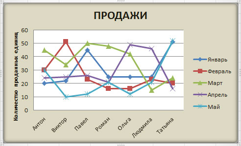
We will build a graph using the example of the following table. We have data about the employees of one of the companies - who sold how many units of goods for a certain month.

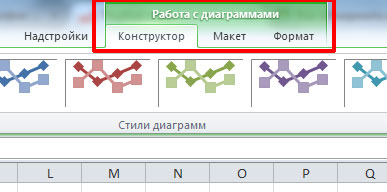
Let's make a graph in Excel that will display the number of units sold by each of the employees in January. Select the corresponding column in the table, go to the "Insert" tab and click on the button "Graph". Choose one of the suggested options. For each chart there is a hint that will help you decide in which case it is best to use it. We use "Graph with markers".

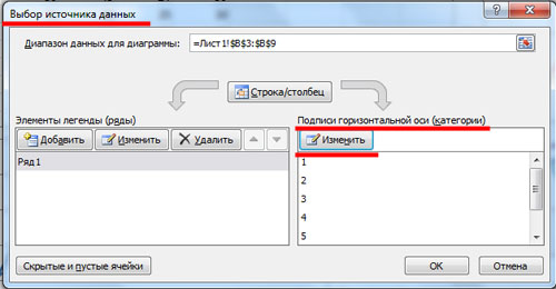
This is the chart we got. Let's change the labels on the horizontal axis: instead of numbers, put the names of employees. Select the horizontal axis, right-click on it and select from the context menu "Select data".

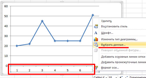
A window will appear "Select data source". In chapter "Horizontal Axis Labels" click on the button "Change".

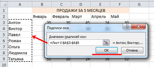
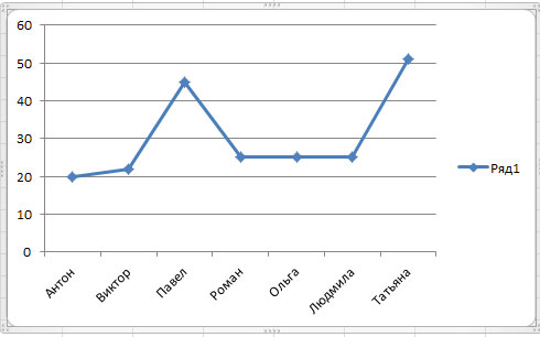
Now it is clear which employee sold how many units of goods in January.

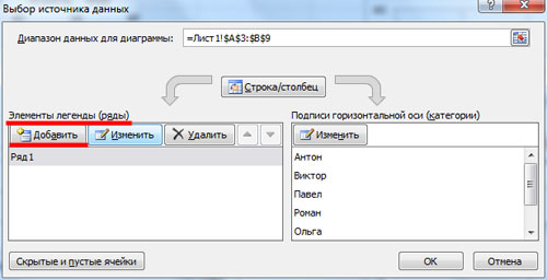
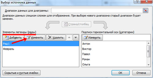
Let's add to the graph, the number of units sold for the remaining months. In the window "Select data source" look at the section "Elements of a Legend" and click on the "Add" button.

We put the cursor in the "Row name" field and select the month in the table - February, go to the "Values" field and select the number of goods sold for February. Changes can be immediately seen on the chart: now there are two charts in the window and a new field in the legend. Click OK.

Do the same for the rest of the months.

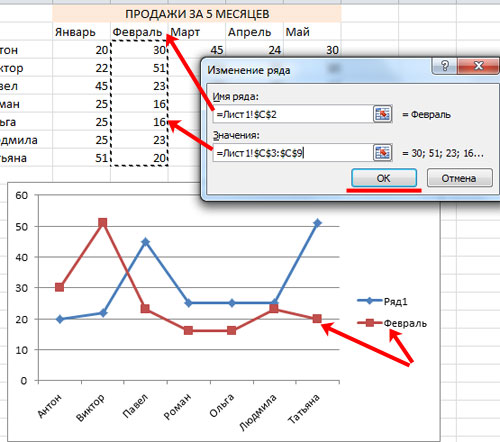
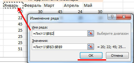
To change the inscription in the legend from "Row 1" to "January", in the window "Select data source" In chapter "Elements of a Legend" select the field "Row 1" and click "Edit".

In the next window, in the field "Series name" put the cursor and select the cell on the sheet with the mouse "January". Click OK.

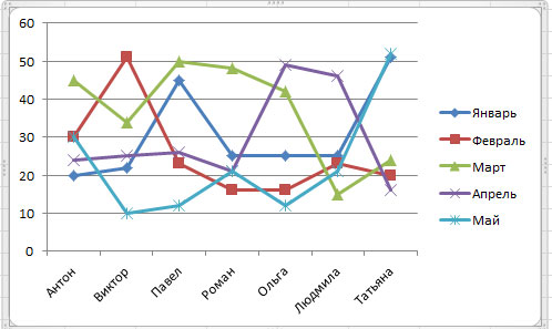
As a result, we get the following graph. It shows in which month, which employee sold the most goods.

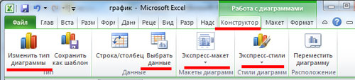
When a chart is selected, new tabs appear on the ribbon for working with charts: "Designer", "Layout" and "Format".

On the tab "Designer", you can change the type of chart, choose one of the proposed layouts and styles. There is also a button already familiar to us. "Select data".

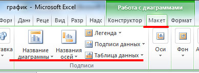
On the Layout tab, you can add a chart title and axis titles. Let's call the chart "Sales", and the vertical axis - "Number of Units Sold". Let's leave the legend on the right. You can enable data labels for plots.

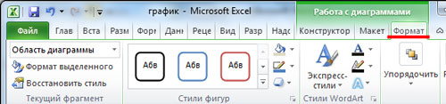
On the "Format" tab, you can choose the fill for the chart, the color of the text, and more.

Format the graph as you wish, well, or according to certain requirements.

This is how easy it is to build a graph on a table with data that changes over time in Excel.